Essay 4.4 Bayesian Analysis: From Metaphor to Formal Model

n Chapter 4 of the textbook, “perceptual committees” in middle vision was discussed. While we hope that is a useful way to think about what’s going on, it is just a metaphor. There are formal, mathematical ways to model the way in which knowledge about regularities in the world can constrain the interpretation of ambiguous sensory input. One of the most fruitful approaches is known as the Bayesian approach (Kersten et al., 2004; Yuille and Kersten, 2006). Thomas Bayes (1702–1761), an eighteenth-century Presbyterian minister, was the first to describe the relevant mathematics.

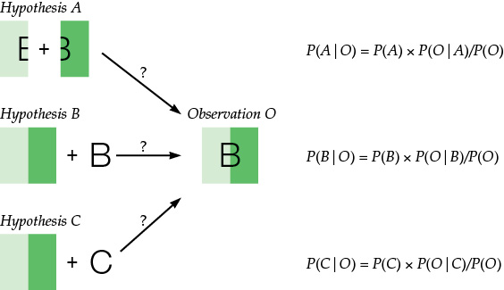
The image above is a version of textbook Figure 4.35. Here, we retell the story of that figure with a bit more formal detail. Our visual system looks at the stimulus and makes an observation (call it “O”). Suppose we wanted to make our best guess as to what situation in the real world produced that observation. Let’s consider three hypotheses, illustrated in the figure: hypothesis A says that we’re looking at two green rectangles. The light one has a narrow letter E on it, and the dark one has a narrow numeral 3. These just happen to precisely line up in order to produce a B like the one we observed. Hypothesis B says we’re looking at a green square—half light and half dark green—with a B on it. Hypothesis C says we’re looking at the same green square, but it really has a C on it. Of course, an infinity of other hypotheses could be entertained here (it’s really a chicken, it’s really dinner, and so on), but these three will do as representatives.

Which hypothesis represents the most likely explanation of the observation? We can represent the likelihood of hypothesis A as P(A|O), which we would read as the probability of hypothesis A, given observation O. We want to know which probability is the highest: P(A|O), P(B|O), or P(C|O). Bayes’ theorem gives us a way of computing these probabilities. Specifically, the theorem says:

P(A|O) = P(A) × P(O|A)/P(O)

Let’s unpack this equation a bit. P(A) is the probability that hypothesis A ever happens. Which hypothesis would we think was correct if we had our eyes closed and never made observation O? We don’t know precisely, but given what we know about the world, we can assume that both P(B) and P(C) are likely bigger than P(A), since hypothesis A relies on a very precise and therefore unlikely alignment of a skinny E with a skinny 3. This first term is what is known as the prior probability; the probability that a given hypothesis is correct before any observations are made.

The second term, P(O|A), asks—if a given hypothesis is correct—how likely we were to make the observation O. In the figure, hypotheses A and B are likely to lead to observations much like O. Hypothesis C is unlikely. (What are the chances that the letter looks like a B but it is really a C?) So, P(O|A) and P(O|B) are both larger than P(O|C).

The third term, P(O), asks—of all possible observations we could possibly have made, anywhere in the world—what’s the probability of observing O? This number can be difficult to calculate, but thankfully it’s the same for all three hypotheses, so we can ignore the effects of P(O).

What, then, is our best guess about the situation in the real world? Hypotheses B and C have better prior probabilities: P(B) and P(C). Hypotheses A and B have better likelihoods: P(A|O) and P(B|O). Overall, the Bayesian approach will tell us that hypothesis B is a better bet than either hypothesis A or hypothesis C (and all those chicken and dinner hypotheses are vastly unlikely).

References

Kersten, D., Mamassian, P. and Yuille, A. (2004). Object perception as Bayesian inference. Annu Rev Psychol, 55, 271–304.

Yuille, A. and Kersten, D. (2006). Vision as Bayesian inference: Analysis by synthesis? Trends Cogn Sci, 10, 301–308.